A Simple Example

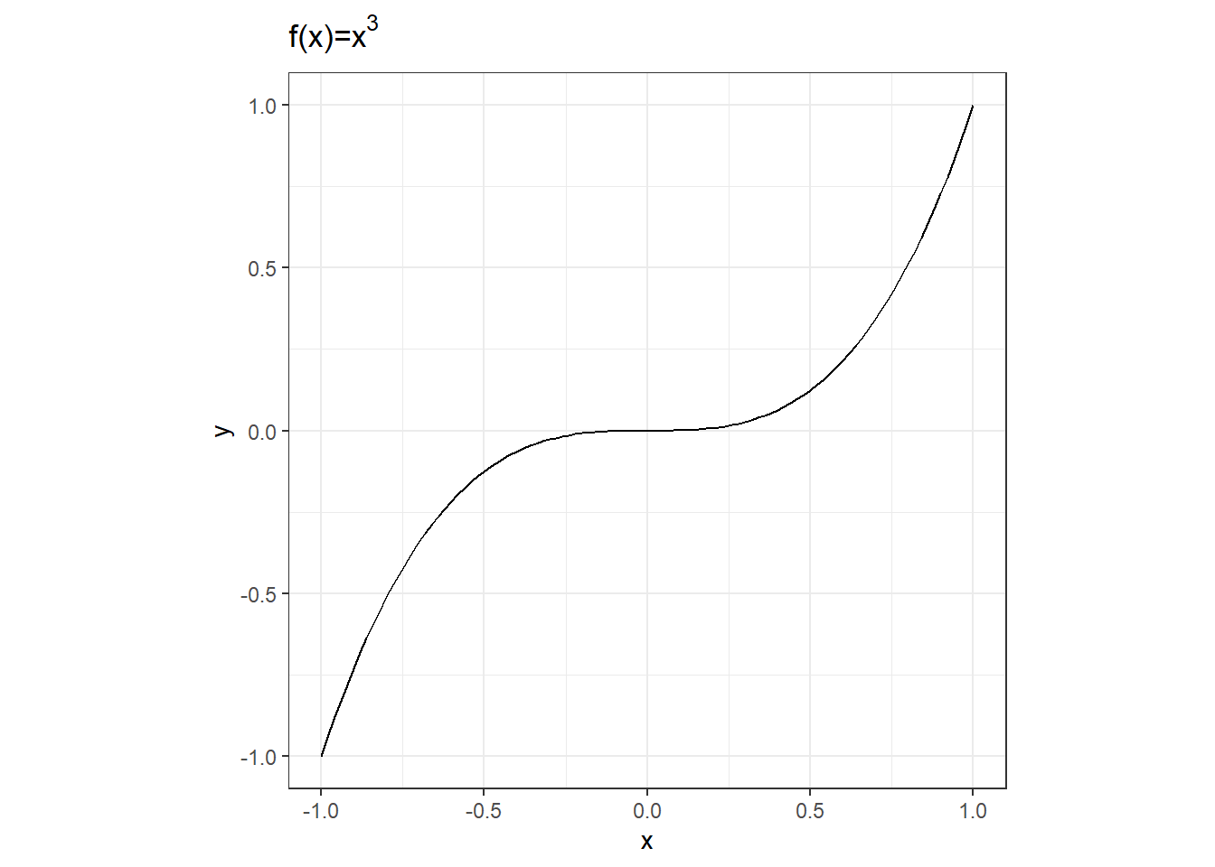
Let’s say your function is the cubic \(f(x) = x^3\) and you want to know where \(f(x) = 0\) (we will look at other values later), or in other words, where the root of the function is. First, let’s take a look at the plot.

Wow, pretty boring and obvious that \(x=0\) when \(y=0\). But how would we find this with R? R has a function called uniroot specifically designed to find roots of a function. To work correctly, uniroot needs an interval that it will search within. From our plot, we can see that the root is within \(x=-1\) and \(x=1\).

cubic <- function(x) {
  x^3
}
uniroot(f = cubic, interval = c(-1,1)) %>% 
  str()

#> List of 5
#>  $ root      : num 0
#>  $ f.root    : num 0
#>  $ iter      : int 1
#>  $ init.it   : int NA
#>  $ estim.prec: num 1

Besides the root we are looking for, uniroot returns a list of a few other things, f.root gives us the value that cubic(root) would produce (useful for seeing how accurate uniroot was able to get). iter is the number of iterations that it took to find the root. More details about these are in the documentation.

If we give the function an interval that does not contain the root we will get the following.

uniroot(f = cubic, interval = c(.5,1))

#> Error in uniroot(f = cubic, interval = c(0.5, 1)): f() values at end points not of opposite sign

So earlier I actually wasn’t specific enough. Not only does interval need to contain the root, but also the function values at the endpoints need to have opposite signs. Stated differently, the interval \([a,b]\) that contains the root must satisfy \(f(a)f(b) < 0\).

Non-root Solving

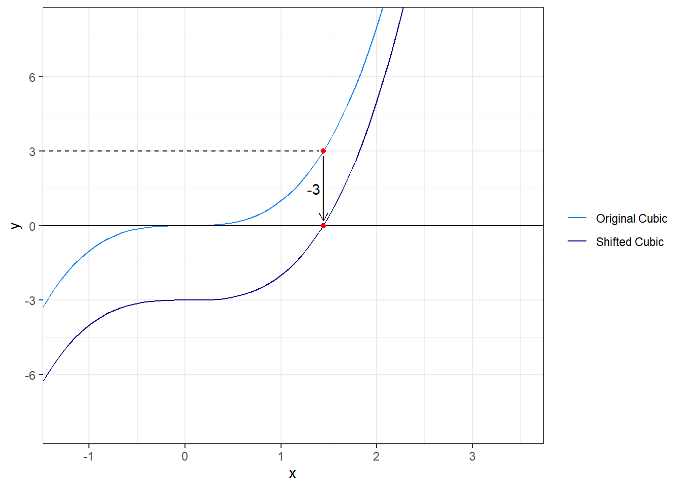
uniroot solves for roots (where \(f(x) = 0\)) but many times we are looking for other values (where \(f(x) \ne 0\)). The trick to use uniroot for other values is to vertically shift the function we are solving so that solving for the root of the shifted function will give us the value we want. Now considering the same cubic function, let’s say we want to know where \(f(x) = 3\). If we subtract 3 from the function we create a new function where the root has the same \(x\) value as the solution of \(f(x) = 3\). We can then solve for the root just as we did before.

Let’s look at a graph of this.

From the graph we know a good interval to use and we can now solve.

cubic_shift <- function(x) {
  cubic(x) - 3
}
uniroot(cubic_shift, c(1,2))$root

#> [1] 1.442242

Example Use Case

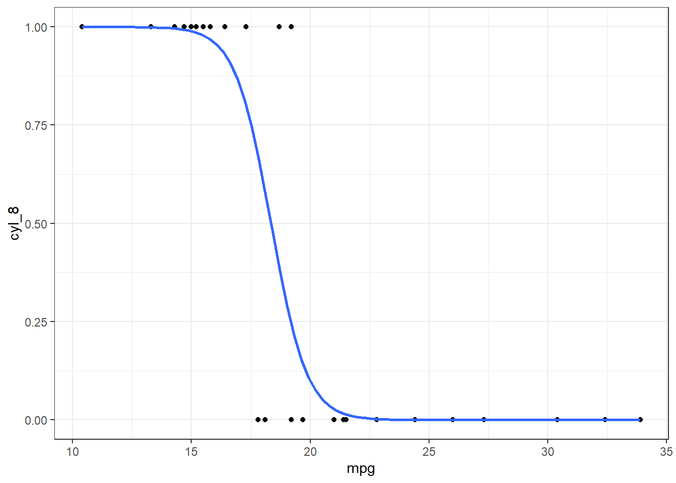
Here I will show you how I have used uniroot recently and how you might make use of it. We will use uniroot to find where there is a probability of 50% in a logistic regression. First, we will create some toy data appropriate for a logistic regression and we will take a look at a graph of the model.

library(ggplot2)
library(dplyr)

mt_dat <- mtcars %>%
  mutate(cyl_8 = as.numeric(cyl == 8))

mt_plot <- mt_dat %>%
  ggplot(aes(mpg, cyl_8)) +
  geom_point() +
  geom_smooth(se = F,
              method = "glm",
              method.args = list(family = "binomial")) +
  theme_bw()
mt_plot

It looks like within this sample there is a 50% probability of a car having 8 cylinders when the car gets somewhere between 17.5 and 20 miles-per-gallon (see ?mtcars). To get a more accurate value, we will first need to create the model for this situation.

mt_model <- glm(cyl_8~mpg, family = "binomial", data = mt_dat)

In this case, we could pull out the coefficients from mt_model and use those to create the logistic function and solve like we did before. However a simpler solution is to use predict by making a helper function called prob_root that will use predict inside of it.

Note that prob_root has no meaning in the context of this problem. It’s just a function that we need to create for uniroot just like the shifted cubic before.

prob_root <- function(x, prob) {
  (predict(mt_model,
           # pass the variable we are solving for
           data.frame(mpg = x), 
           type = "response") 
   - prob) # subtract the probability we are looking for 
           # to shift the function just like we did before
}

Two things to keep in mind as you are creating these helper functions:

• The input variable you are solving for should always be the first argument.
• Any additional arguments that are needed for your helper function can be passed from uniroot (in this case the argument prob).

Now that we have created our helper function for uniroot we can solve.

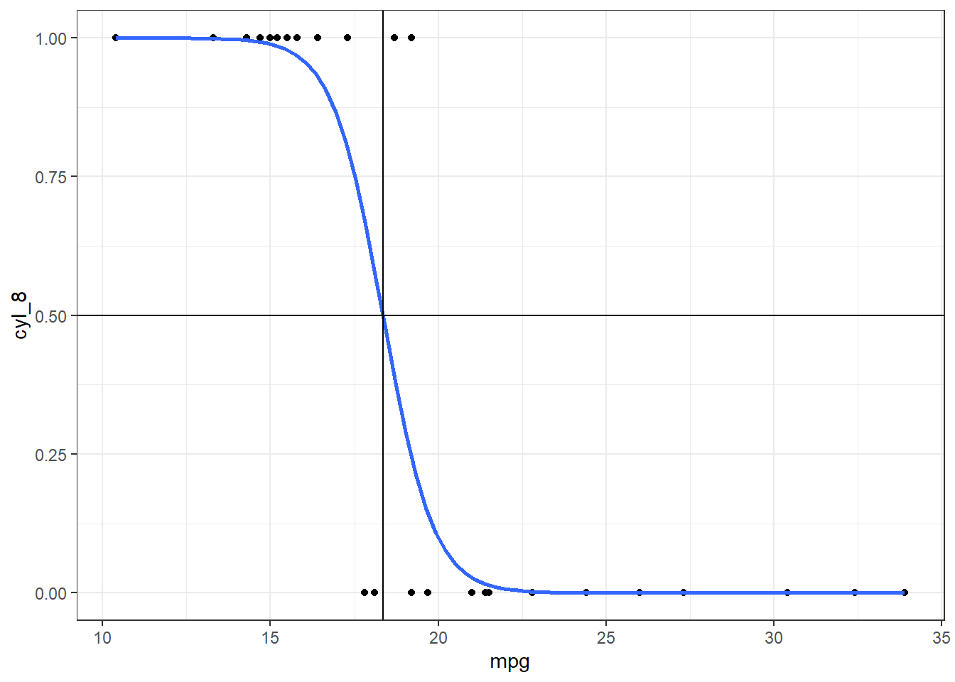
uniroot(prob_root, interval=c(17.5, 20), prob = .5)$root

#> [1] 18.34663

Let’s visually verify our solution.

mt_plot +
  geom_hline(yintercept = .5) +
  geom_vline(xintercept = 18.34663)

---

Thanks for reading! I hope this post helped you understand how to use uniroot and how it can be used in your future projects.