This post is a detailed explanation of my senior project and the process I went through. If you are looking for a broad overview of my project you can check out a poster I made here. If you wish to continue reading but haven’t been introduced to my project yet, read this post and come back here.
Choosing a Model for Estimating R50
When first looking at this problem and the data I was given I knew that a logistic regression could be used to estimate R50. I decided that a good estimate of R50 is the range where there is a 50% probability a target will be detected since R50 is the range where 50% of the targets will be detected. However, a prediction using a logistic model can’t estimate R50 directly. Logistics output a probability given a continuous variable, whereas what I needed was the opposite. I researched to see if there was a way to create a model that would be able to do this “out-of-the-box” but I found nothing. I decided to use the logistic model and find a way to solve for R50 using that model. I will explain this method later.
I chose to create a logistic model using the R package parsnip since prediction output is in a dataframe and I could obtain confidence intervals easily from the model as well.
At first while creating my model, I included the interaction term range:turbines. This would account for a difference in the rate the detection probability changes as the range of the target increases. Below is how I created the model and the estimates of the model’s terms.
logistic_reg() %>%
  set_engine("glm") %>%
fit(as.factor(detection) ~ range * turbines, data = sample)| term | estimate | std.error | statistic | p.value |
|---|---|---|---|---|
| (Intercept) | 6.97 | 2.13 | 3.27 | 0.0011 |
| range | -0.35 | 0.11 | -3.32 | 0.0009 |
| turbines | -3.65 | 2.47 | -1.48 | 0.1392 |
| range:turbines | 0.12 | 0.13 | 0.94 | 0.3496 |
However, the interaction term was not significant so I simplified the model as shown below. All the terms of this model were significant and this was my final choice for a model.
R50_mod <- logistic_reg() %>%
  set_engine("glm") %>%
fit(as.factor(detection) ~ range + turbines, data = sample)| term | estimate | std.error | statistic | p.value |
|---|---|---|---|---|
| (Intercept) | 5.64 | 1.29 | 4.38 | 0.000012 |
| range | -0.28 | 0.06 | -4.70 | 0.000003 |
| turbines | -1.47 | 0.69 | -2.12 | 0.033855 |
Solving for R50 and Confidence Intervals
Since my model couldn’t estimate R50 directly, I created a function solve_R50 that could use the model to solve for R50 and the confidence intervals under each condition. solve_R50 first creates a function R50_root that will have a root at where R50, the upper bound, or the lower bound is (depending on type). It then solves for the root using uniroot for each turbine condition. If you are interested, I wrote a detailed blog post here on the bulk of the logic behind this.
In the function below, the argument R50_mod is the parsnip logistic model and turbines is a binary vector indicating the condition to predict under. The argument type is one of "pred", "lower" or "upper". "pred" gives the predicted R50 value. "lower" or "upper" give the corresponding side of the confidence interval. To see the full function see here.
solve_R50 <- function(R50_mod, turbines, type) {

  # ... skipped logic for `type` argument

  # create a function that we will find the root of using `uniroot`
  R50_root <- function(range, turbines) {
    predict.model_fit(R50_mod,
                      tibble(range = range, turbines = turbines),
                      # pred_type variable determines if we are solving
                      # for R50 or a confidence interval
                      type = pred_type
    ) %>%
      # pick the column we need from predict.model_fit
      # subtracting .5 creates a root where we want it
      pull(pred_col) - .5
  }

  # solve for each `turbines` condition
  map_dbl(turbines,
          ~ uniroot(R50_root,
                    interval = range(R50_mod$fit$data$range),
                    turbines = .x)$root)
}
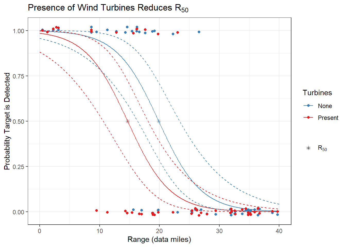
This is how I used the solver to obtain R50 and the confidence intervals for each turbine condition. Below is the information presented in table form and graphically.
R50_dat <-
  tibble(turbines = 0:1) %>%
  mutate(R50 = solve_R50(R50_mod, turbines, "pred"),
         lower = solve_R50(R50_mod, turbines, "lower"),
upper = solve_R50(R50_mod, turbines, "upper"))| Turbines | \(R_{50}\) | Lower | Upper |
|---|---|---|---|
| None | 19.88 | 16.35 | 23.37 |
| Present | 14.68 | 10.59 | 18.09 |

Impact of Wind Turbines on R50
We can determine whether the presence of wind turbines affects R50 by looking at the impact the turbines term has on the model. Below are the estimates of the model’s terms. Since the turbines term is significant and it represents a horizontal shift in the two curves as shown above, the estimated R50 will be significantly different under the two conditions. In this sample, the presence of wind turbines reduced R50 by 5.2 data miles.
| term | estimate | std.error | statistic | p.value |
|---|---|---|---|---|
| (Intercept) | 5.64 | 1.29 | 4.38 | 0.000012 |
| range | -0.28 | 0.06 | -4.70 | 0.000003 |
| turbines | -1.47 | 0.69 | -2.12 | 0.033855 |
Estimation of Power
To calculate power I needed to estimate the standard deviation of R50. I used the confidence intervals to make this estimation. Unfortunately, the confidence intervals were not symmetric after translating them to be in terms of range. More specifically, the distance from R50 to the upper bound was not equal to the distance from R50 to the upper bound. To be conservative in the power calculations I choose the largest margin to determine the standard deviation.
| Turbines | \(R_{50}\) | Lower | Upper | Lower Margin | Upper Margin |
|---|---|---|---|---|---|
| None | 19.88 | 16.35 | 23.37 | -3.53 | 3.50 |
| Present | 14.68 | 10.59 | 18.09 | -4.09 | 3.41 |
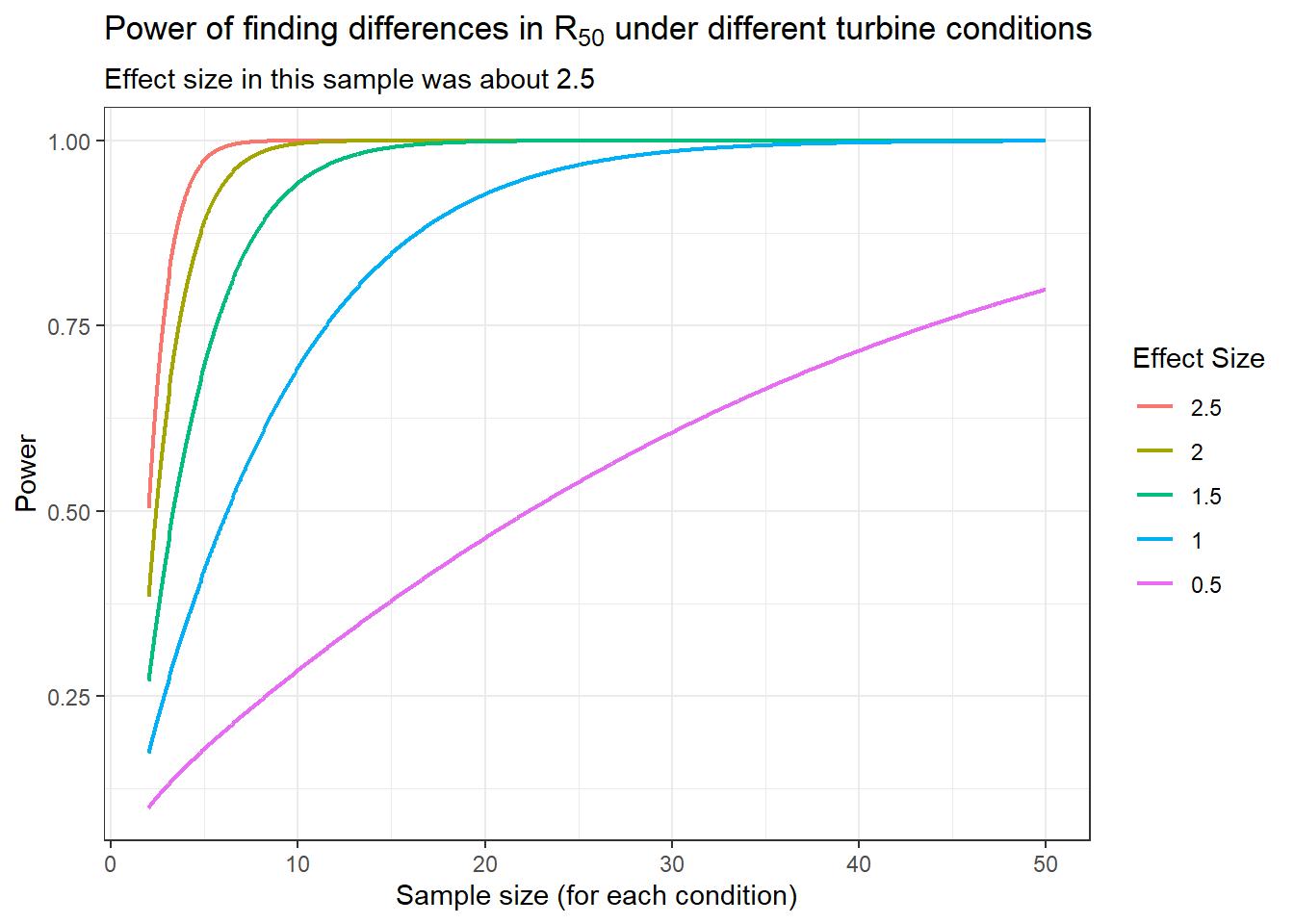
Assuming there are two standard deviations from R50 to the interval bounds, my over-estimate for the standard deviation is about 2 (4.09 / 2). Since the difference in the R50 estimates is about 5 data miles when there are wind turbines versus no turbines, then the estimates are about 2.5 standard deviations from each other. In other words, the effect size is about 2.5 in this sample.
To calculate power across different sample sizes and effect sizes I used the function pwr.t.test from the R package pwr. Using a function normally used for t-test power calculations made sense in this situation because if R50 was estimated from several different samples of data under both turbine conditions, then a t-test would be used to compare the two sets of R50 estimates to prove that R50 is different under those conditions. Below is a power curve plot made using pwr.t.test for effect sizes and sample sizes smaller than the one in this sample.

Goals Accomplished
By the end of this project, I developed a model and a method for estimating R50 and I estimated the confidence intervals of R50. I also identified the impact of the presence of wind turbines on R50 and I estimated the power of finding this impact for different sample sizes and effect sizes. If desired the code for this project can be found here.